%%TRABAJO MATLAB

%%DIEGO DAVID MONTENEGRO TAMA

%%EJERCICIO 1
%Ejercicio 1 apartado a
type combina
%%Ejercicio 1 apartado b
type bernstein
%Ejercicio 1 apartado c
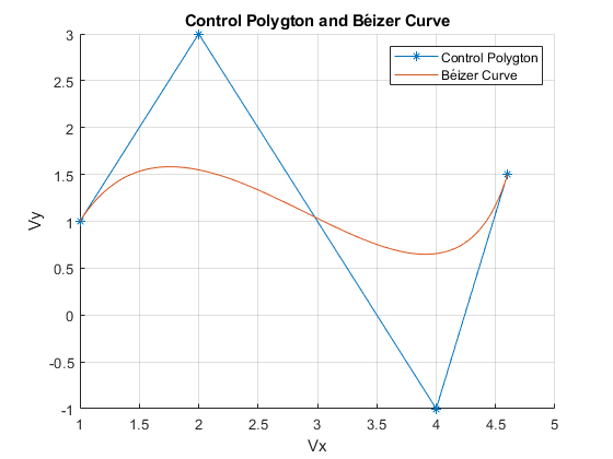
figure(1)
t=linspace(0,1);
V=[1 2 4 4.6;1 3 -1 1.5];
hold on
plot(V(1,:),V(2,:),'-*');
grid on
n=size(V);
n=n(2);
hold off
s=size(t);
x=zeros(n,s(2));
y=zeros(n,s(2));
for i=1:n
    x(i,:)=bernstein(n-1,i-1,t)*V(1,i);
    y(i,:)=bernstein(n-1,i-1,t)*V(2,i);
end
hold on
a=sum(x);
b=sum(y);
hold on;
plot(a,b);
%Añadimos:Titulo,leyenda y titulo en los ejes
titulo='Control Polygton and Béizer Curve';
legend('Control Polygton','Béizer Curve');
title(titulo)
xlabel('Vx')
ylabel('Vy')
hold off
clear,clc

function resultado = combina(n,i)
resultado = factr(n)/(factr(i)*factr(n-i));
end


function bn = bernstein(n,i,t)
bn = combina(n,i)*t.^i.*(1-t).^(n-i);
end

%%EJERCICIO 2

%%Ejercicio 2 apartado a)
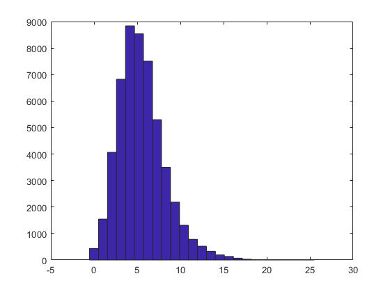
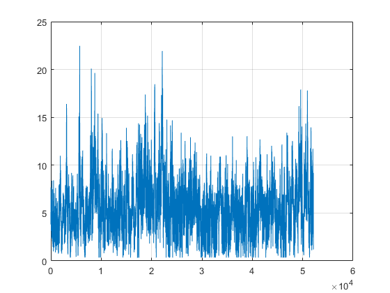
dw=xlsread('sotaventogaliciaanual.xlsx');
nbins=linspace(0,25,25);
figure(1)
hist(dw,nbins)
figure(2)
plot(dw)
grid on
clear,clc

%%Ejercicio 2 apartado b)
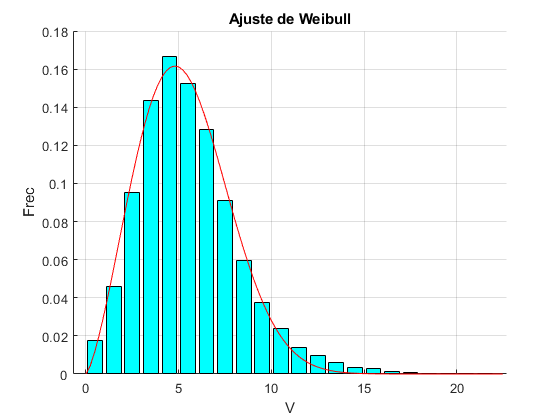
Y=xlsread('sotaventogaliciaanual.xlsx','B:B');
x=0.5:1:max(Y);
viento=hist(Y,x,'r');
frec=viento/sum(viento);
f=@(a,x) (a(1)/a(2))*((x/a(2)).^(a(1)-1)).*exp(-(x/a(2)).^a(1));
k=std(Y);
c=mean(Y);
a0=[k c];
af=nlinfit(x,frec,f,a0);
figure(3)
hold on
bar(x,frec,'c');
x=linspace(0,max(Y),100);
y=f(af,x);
plot(x,y,'r')
grid on
title('Ajuste de Weibull')
xlabel('V')
ylabel('Frec')
hold off

%%Ejercicio 2 apartado c)
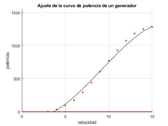
Pr=1300; x0=3.0;xr=20;x1=25; %datos de la curva de potencia
k=2.3849; c=6.0208; %parametros weibul calculados anteriormente
potencia=xlsread('sotavento_curva potencia.xlsx','B2:B27');
x=0:1:25;
pot=potencia(x>=x0 & x<=xr);
hold on
x=x0:1:xr;
grid on
plot(x,pot,'ro','markersize',3,'markerfacecolor','r')
title('Ajuste de la curva de potencia de un generador');
axis([0 15 -10 1550])
xlabel('velocidad')
ylabel('potencia')
grid on

%ajuste
p=polyfit(x,pot',3); %ajuste a un polinomio cúbico
yp=polyval(p,x);
plot(x,yp,'k')
hold off
clear,clc

%%Ejercicio 3
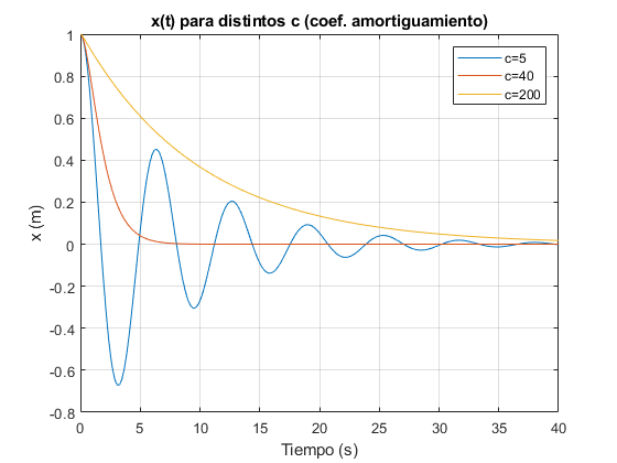
[t1, xx1]=ode45(@muelle, [0,40], [1,0],[ ], 5);
plot(t1,xx1(:,1))

hold on

[t2, xx2]=ode45(@muelle, [0,40], [1,0],[ ], 40);
plot(t2,xx2(:,1))
grid on;
[t3, xx3]=ode45(@muelle, [0,40], [1,0],[ ], 200);
plot(t3,xx3(:,1))
xlabel('Tiempo (s)');
ylabel('x (m)');
title('x(t) para distintos c (coef. amortiguamiento)');
legend('c=5','c=40','c=200');

% funcion muelle
function x=muelle(t,x,c)
x=[x(2); (-c*x(2)-20*x(1))/20];
end

Published with MATLAB® R2019a